This is a reference workflow for differential abundance analysis, using a simple experiment comparing protein abundances across two cell lines (SS6 and SS48) with triplicate measurements. Workflow and code can be adapted to a wide range of proteomics experiments, such as time series or affinity purification experiments.
How to follow this vignette
Copy the R code chunks and run them locally as you go through this document. You should already be familiar with R data.table and ggplot. The input file protein_quant.csv.gz is produced by the DIA-NN data processing tutorial. The source code for this whole document is accessible through the Code button in the top right.
1 Preparing the data
We start with a data table of protein identifiers (e.g. Protein_group) and their quantities (e.g. LFQ) across samples. Initially, we prepare the data for downstream analysis (e.g. log2 transformation).
Code
# Load required librarieslibrary(data.table); library(ggplot2); library(ggupset); library(patchwork); library(imputeLCMD); library(limma); library(highcharter)# Make script execution reproducibleset.seed(123)# Set a plotting theme for the whole documenttheme_set( theme( text =element_text(size =8), panel.border =element_rect(linewidth =0.25, colour ="black", fill =NA), panel.background =element_blank(), panel.grid =element_blank(), axis.text =element_text(colour ="black"), strip.background =element_blank(), strip.text =element_text(size =8, vjust =1)))# Load protein quantitationsDT <-fread("protein_quant.csv.gz")# Select a protein quantitation column (e.g. LFQ) and log2-transform itDT <- DT[, log2_quant :=log2(LFQ) ]# Print selected columnsDT[1:5, .(Sample, Protein_group, log2_quant)]
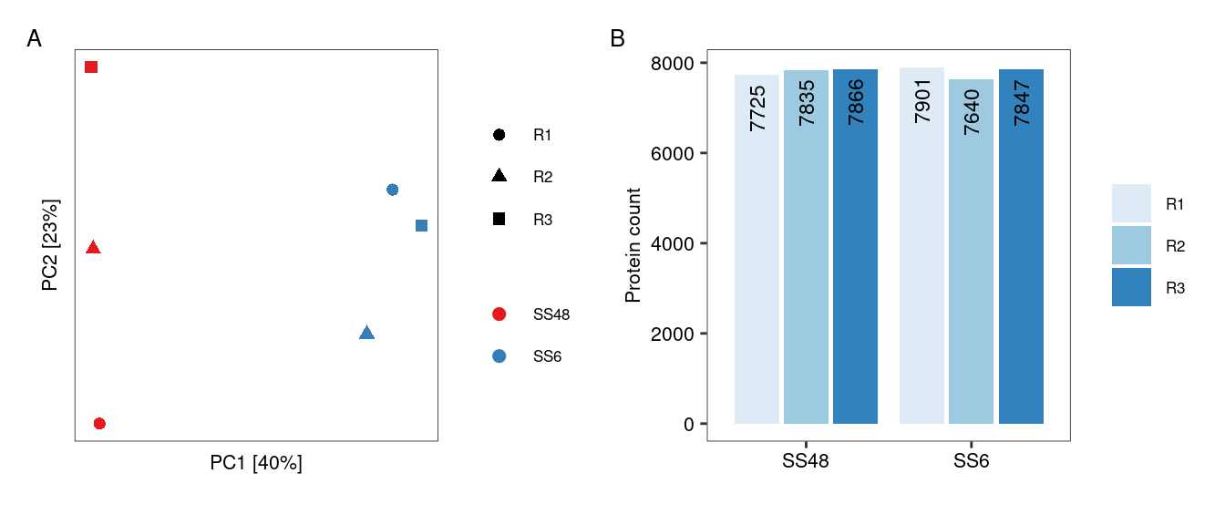
Occasionally, an MS run may yield poor results, for example due to material loss during the sample prep. While we typically identify such outliers earlier in the data processing pipeline, it is good practice to perform a PCA analysis to identify any samples that deviate unexpectedly. Another flag for problematic runs is a severe drop in the number of quantified proteins. As shown by Figure 1, there are no obvious outliers in this dataset and no samples need to be excluded.
Code
# Run a PCA to check for major trendsPCA_input <-dcast(DT, Protein_group ~ Sample, value.var ="log2_quant") # Cast into a wide data format for PCA analysisPCA_input <- PCA_input[ complete.cases(PCA_input) ] # Can't do PCA with missing valuesPCA_input <-t( data.frame( PCA_input, row.names ="Protein_group" )) # Convert to dataframe and transpose to compare samplesDT_PCA <-prcomp( PCA_input , scale. =TRUE ) # Run PCAvar_explained <-summary(DT_PCA)$importance # Extract variance explainedDT_PCA <-data.table(DT_PCA$x, keep.rownames ="Sample") # Prepare for plottingDT_PCA <-merge(DT_PCA, unique(DT[, .(Sample, Condition, Replicate)])) # Add annotation of conditions and replicates# Create PCA plotpPCA <-ggplot(DT_PCA, aes(x = PC1, y = PC2, colour = Condition, shape = Replicate))+geom_point( size =2 )+scale_colour_brewer(palette ="Set1")+xlab(paste("PC1 [", round( var_explained[ rownames(var_explained) =="Proportion of Variance" , "PC1"] *100, 0), "%]", sep =""))+ylab(paste("PC2 [", round( var_explained[ rownames(var_explained) =="Proportion of Variance" , "PC2"] *100, 0), "%]", sep =""))+theme(axis.text =element_blank(), axis.ticks =element_blank(), legend.title =element_blank())# Create barplot with number of remaining proteins per samplepBar <-ggplot( DT[, .N, .(Condition, Replicate)], aes( x = Condition, y = N, fill = Replicate, label = N))+geom_bar(stat ="identity", position ="dodge2")+geom_text(position =position_dodge2(width =0.9), vjust =0.5, hjust =1.2, size =3, angle =90)+scale_fill_brewer()+labs(x =NULL, y ="Protein count", fill =NULL)# Arrange the two plots into a single figure using the Patchwork packagefree(pPCA, type ="label") + pBar +plot_annotation(tag_levels ="A")
Figure 1: Inspecting dataset for outlier samples. (A) PCA shows that replicates group together as expected. (B) Bar chart shows consistent number of proteins identified across replicates.
2.2 Proteins
We filter out proteins with insufficient or unreliable quantitation, aiming to retain as many as possible for downstream analysis while minimising noise from inconsistently measured proteins. There is no single filtering strategy that will work for all datasets. The filtering strategy needs to be tailored to the data and the downstream analysis. Generally, it helps to consider both quality (e.g. number of precursors) and frequency (e.g. number of replicates) of protein quantitations.
This particular dataset has six samples. We filter it as follows:
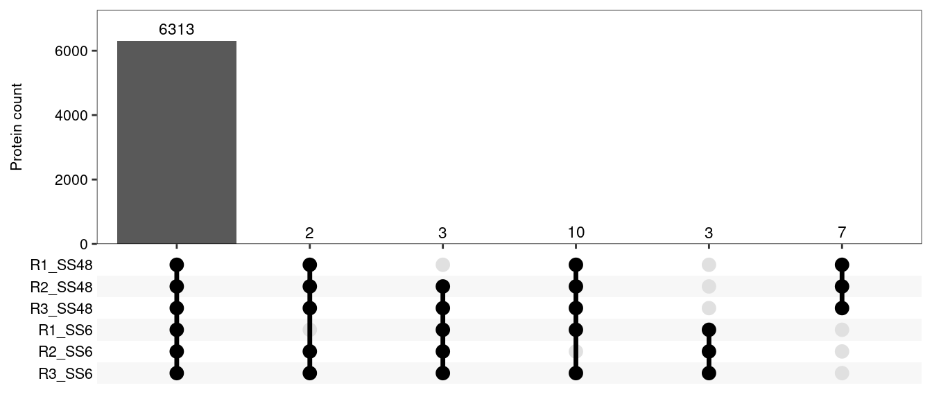
Keep proteins detected in all 6 samples with at least 2 precursors (n = 6,310).
Keep proteins detected in 5 samples with at least 3 precursors. We can still calculate fold-changes and p-values for these proteins, but significance will be reduced due to the missing replicate in one condition. The stricter precursor threshold reduces the risk of retaining spurious hits (n = 13).
We cannot keep proteins detected in ≤4 samples, because the resulting statistical analysis would be unreliable. An important exception is when a protein is consistently quantified in all replicates of one condition but entirely absent in the other. This could be a truly condition-specific expression profile, or a highly specific interaction in an IP compared to an IgG control. In such cases, we can impute a baseline value for the missing condition, allowing us to calculate a fold-change for statistical analysis (see imputation section). Any such fold-change will be a conservative estimate compared to the “infinite” fold-change implied by a complete absence in one condition. To capture this third group, we keep proteins detected in 3 samples with at least 5 precursors, but only if the three samples belong to the same condition, and only if they were not detected at all in the other condition (n = 9).
After filtering, let’s see how many proteins we have left to work with:
Code
# Calculate protein stats before filteringprotein_stats <- DT[, .(n_samples = .N, # Number of samplesmin_precursors =min(N_precursors), # Mininum number of precursors across samplesn_conditions =uniqueN(Condition) # Number of different conditions ), Protein_group ] # Calculate for each protein# Proteins detected in 6 samples with at least 2 precursorskeepers_1 <- protein_stats[ n_samples ==6& min_precursors >=2, Protein_group ]# Proteins detected in 5 samples with at least 3 precursorskeepers_2 <- protein_stats[ n_samples ==5& min_precursors >=3, Protein_group ]# Proteins detected in 3 samples with at least 4 precursors, but these samples are from a single condition, and the protein has not been detected at all in the other conditionkeepers_3 <- protein_stats[ n_samples ==3& min_precursors >=5& n_conditions ==1, Protein_group]# Filter table to keep only these three sets of proteinsDT <- DT[ Protein_group %in%c(keepers_1, keepers_2, keepers_3) ]# Create UpSet plot to show protein overlap between sample pairspUpSet <-ggplot( DT[, .(Sample =list(Sample)), by = Protein_group], # Prep data for ggupset's scale_x_upset functionaes(x = Sample))+geom_bar()+geom_text(stat='count', aes(label =after_stat(count)), vjust =-0.5, size =3) +# This adds protein numbers on top of the barsscale_x_upset(order_by ="degree", reverse =TRUE, sets = DT[ order(Condition), unique(Sample)] )+# Explicitly providing the set names allows us to order them by conditionlabs(x =NULL, y ="Protein count")+scale_y_continuous(expand =expansion(mult =c(0,0.15))) # This expansion is necessary to accomodate numbers on top of bars# Output plotpUpSet
Figure 2: Protein numbers after filtering, and their overlap across samples.
3 Normalisation
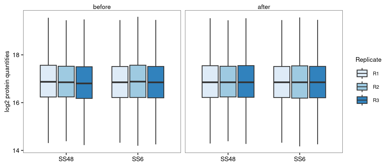
These data have already been normalised at the precursor level to adjust for unequal sample loading. Additional normalisation steps are often not required. In fact, some sophisticated normalisation procedures used in the field are actually reducing workflow performance (Peng et al. 2024). Nevertheless, for many experiments we can assume that most protein abundances do not change between conditions, so we set the median protein abundance to the same value across all samples.
Code
# Identify the "median of the medians". This will become the new median for all samples.target_median <- DT[, median(log2_quant), Sample][, median(V1)]# Scale protein quantities to obtain this target_median for all samplesDT[, log2_quant_norm := log2_quant -median(log2_quant) + target_median, by = Sample] # Plot the values before and after the median normalisationpBar <-ggplot( data =melt(DT, measure.vars =c("log2_quant", "log2_quant_norm")),aes(x = Condition, fill = Replicate, y = value))+facet_wrap("variable", labeller =labeller(variable =c("log2_quant"="before", "log2_quant_norm"="after")))+geom_boxplot(outliers =FALSE)+scale_fill_brewer()+labs(x =NULL, y ="log2 protein quantities")# Output plotpBar
Figure 3: Boxplot showing protein quantities before and after median-normalisation. Median normalisation helps to make sure that the median fold-change between conditions is zero.
4 Missing value imputation
Missing values are common in proteomics and many algorithms exist to impute them. However, imputation should be used very cautiously. Most missing values in proteomics are missing for a reason, typically because low-abundance proteins are inconsistently quantified across samples. In many cases, imputation is not necessary. For example, proteins quantified in 5 samples in this dataset (keepers_2) are missing from one replicate in one condition. We can calculate differential expression p-values for such proteins (see below), which will be less significant than for comparable proteins with a full set of replicates. Nevertheless, this is a more robust approach than imputing a value for the missing replicate and feeding it as “real” observation into the differential expression analysis.
However, there is one scenario where imputation is necessary: when a protein is consistently and robustly detected in one condition but entirely absent in another (see protein filtering section). In our dataset we have identified 9 proteins that may considered truly condition-specific (keepers_3). For these proteins, we can impute “baseline” values for the condition in which they are absent, so that we can estimate fold-changes and include them in our downstream analysis.
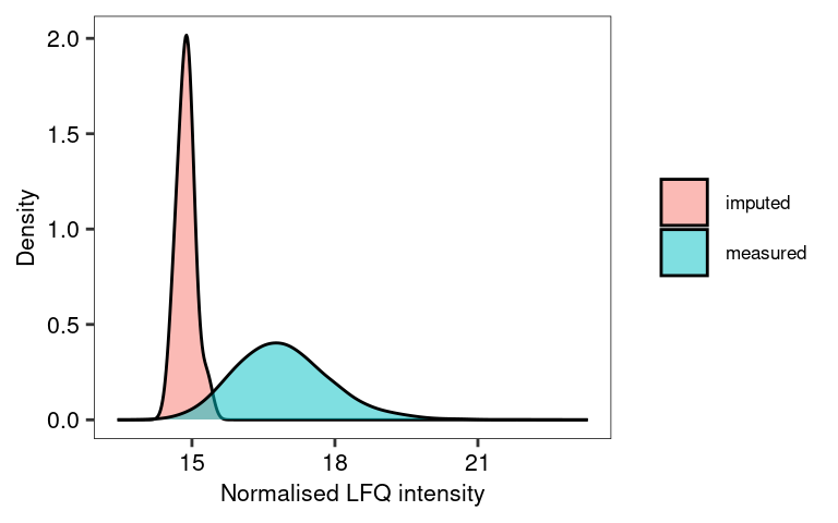
We use the minProb approach, which simulates low-abundance values in a sample- and protein-specific manner (Lazar et al. 2016). Specifically, minProb draws a random value from a normal distribution, where the mean corresponds to the bottom 1% of intensities in the sample. The distribution’s variance is determined by the variability of the protein’s abundances in the samples where it was detected.
Code
# We first need to cast the data into a wide formatwDT <-dcast(DT, Protein_group ~ Sample, value.var ="log2_quant_norm", fill =NA)# Impute missing values wDT_imp <-impute.MinProb( as.matrix(wDT, rownames ="Protein_group"), q =0.01, tune.sigma =1) # Turn imputed data back into a data.tablewDT_imp <-as.data.table(wDT_imp, keep.rownames ="Protein_group")# Create a table that allows the identification of the original and imputed valuesplot_imp_dt <-merge(melt(wDT, id.vars ="Protein_group", value.name ="measured_val" ),melt(wDT_imp, id.vars ="Protein_group", value.name ="imputed_val" ))plot_imp_dt[ is.na(measured_val), data :="imputed" ]plot_imp_dt[ !is.na(measured_val), data :="measured" ]# Visualise the distribution of the imputed data using this tableggplot( plot_imp_dt, aes(imputed_val, fill = data))+geom_density(adjust =2, alpha =0.5)+labs(x ="Normalised LFQ intensity", y ="Density", fill =NULL)
Figure 4: The values imputed by MinProb fall towards the bottom end of the distribution of the measured values. To change the position or width of the imputed data distribution, adjust q and tune.sigma, respectively. Note we only actually impute values for 9 proteins.
Note that wDT_imp contains imputed data for all missing values (we had to supply the whole data set for imputation, because MinProb needs to know the overall distribution of the data). However, we only want to impute the values for proteins that were exclusively detected in one condition, which we had previously defined as keepers_3. We therefore need to swap out that subsection of our data matrix with the corresponding imputed section.
Code
# Make a record of which values exactly were imputedimpNAs <-melt( wDT[ Protein_group %in% keepers_3 ], id.vars ="Protein_group" )impNAs <- impNAs[ is.na(value), .(Imputed_samples =paste(variable, collapse =",")), Protein_group ]# Replace the original values for these proteins with the imputed oneswDT <-rbindlist( list( wDT[ !Protein_group %in% keepers_3 ], wDT_imp[ Protein_group %in% keepers_3 ]), use.names =TRUE )
5 Differential abundance analysis
5.1 Using a t-test
We first calculate log2 fold-changes manually and use a simple t-test to assess if there is a significant difference between the two conditions. This is a straightforward approach, and in many cases it is sufficient.
Code
# Melt the partially imputed data matrix into long-formatmDT <-melt( wDT, id.vars ="Protein_group", value.name ="log2_quant_norm", variable.factor =FALSE, variable.name ="Sample", na.rm =TRUE)# Re-annotate conditionsmDT[, Condition :=gsub("R\\d_", "", Sample)] # Un-log the LFQ intensities to calculate mean and CVsmDT[, quant_norm :=2^log2_quant_norm ]# For each protein and condition, calculate mean, CV and number of replicates per conditionFC <- mDT[, .(log2_mean_LFQ =log2( mean( quant_norm )), # Log2 of arithmetic mean of LFQsCV =sd(quant_norm) /mean(quant_norm) *100, # CV values across replicatesN_replicates = .N # Number of replicates ), .(Protein_group, Condition) ]# Cast back into a wide tableFC <-dcast(FC, Protein_group ~ Condition, value.var =c("log2_mean_LFQ", "CV", "N_replicates"))# Calculate log2 fold-changeFC[, manual_log2_FC_SS6_SS48 := log2_mean_LFQ_SS6 - log2_mean_LFQ_SS48 ]# Calculate p-values for differential abundance using a t.test (it is generally recommended to do this in log-space)pvalues <- mDT[, .(pval_t_test =t.test(log2_quant_norm ~ Condition)$p.value), Protein_group]# Combine fold-changes and p-valuesFC <-merge(FC, pvalues, by ="Protein_group")# Print resulting data frameFC[ 1:5, .(Protein_group, manual_log2_FC_SS6_SS48, pval_t_test, CV_SS6, CV_SS48)]
Limma is a more sophisticated approach for differential expression analysis (Ritchie et al. 2015). Originally developed for microarrays, it offers two key advantages over a t-test. Limma can handle complex experimental setups, such as comparing multiple conditions and time points, and it can even model and adjust for batch effects. In addition, limma performs particularly well in studies with small sample sizes. With only 3-4 replicates, the true expression variation of a gene is difficult to estimate, which can lead to unreliable p-values. Limma addresses this using an empirical Bayes approach to “borrow information” across all genes. This leads to more stable estimates of expression variability, and therefore more reliable identification of differentially expressed genes. Here we outline a basic limma experiment. For more information, see limma vignettes1.
First, we need to create a design matrix. It tells limma which MS runs / samples (rows) belong to which experimental condition (columns). It is a standard numeric matrix in R, with 1 indicating a match, and zero indicating no match. Design matrices can become quite complex for advanced experimental designs.
Code
# Extract a table that maps samples to conditions sample_map <-unique( DT[, .(Sample, Condition)] )# Turn into design matrix of 1s (match) and 0s (no match). The model.matrix function is made for this, but not very intuitive.design <-model.matrix( ~0+ Condition, data = sample_map)# Adjust the column and row namescolnames(design) <-gsub("Condition", "", colnames(design))rownames(design) <- sample_map$Sample# Set the order of the columns in wDT to match the design matrix. This is critical because limma matches them by position, not by namesetcolorder(wDT, neworder =c("Protein_group", sample_map$Sample))# Print design matrixdesign
Next, we fit the linear model. The present data set is very simple, so only one comparison (SS6 vs SS48) is relevant, but for experiments with multiple conditions (e.g. WT, mutant1, mutant2, mutant3), we could extract multiple pairwise comparisons. These comparisons are called contrasts. We can define a set of contrasts of interest using a contrast matrix. For example, the contrast SS6-SS48 will calculate the log2 fold-change and p-values for SS6 / SS48. We then apply the empirical Bayes method to adjust the protein variances (eBayes). Finally, we extract the relevant information from the linear model fit using topTable.
Code
# Fit the linear modelfit <-lmFit(wDT, design)# Define a contrast matrix and extract contrastscont.matrix <-makeContrasts( SS6vsSS48 = SS6-SS48, levels = design)fit2 <-contrasts.fit(fit, cont.matrix)# Borrow information across all proteins to adjust variance estimatesfit2 <-eBayes(fit2)# Extract the limma results, including p-value adjustmentFC_limma <-topTable(fit2, adjust="BH", number =Inf)# Convert the output to data.table, keep and re-name relevant columns and print on screenFC_limma <-as.data.table(FC_limma)FC_limma <- FC_limma[, .(Protein_group, log2_FC_SS6vsSS48 = logFC, p_value = P.Value, adj_p_value = adj.P.Val)]FC_limma[ 1:5 , .(Protein_group, log2_FC_SS6vsSS48, p_value, adj_p_value) ]
We can now combine all results and annotation data to create an overall output file for our differential abundance analysis.
Code
# Merge manual and limma-based differential abundance dataresults <-merge(FC, FC_limma, by ="Protein_group")# Add the annotation about which values were imputedresults <-merge(results, impNAs, by ="Protein_group", all.x =TRUE)# Add gene and protein namesresults <-merge(results, unique( DT[, .(Protein_group, Genes, Protein_description)] ), by ="Protein_group")# Add additional summary statisticssum_stat <- DT[, .( min_N_precursors =min(N_precursors),min_N_precursors_proteotypic =min(N_precursors_proteotypic) ), .(Protein_group, Condition)]sum_stat <-dcast(sum_stat, Protein_group ~ Condition, value.var =c("min_N_precursors", "min_N_precursors_proteotypic"))results <-merge(results, sum_stat, by ="Protein_group", all.x =TRUE)# Extract gene-level UniProt IDs to merge the data with gene-level annotation later on.# This means removing protein isoform information. Gene-level IDs are not unique.results[, gene_group :=sapply(strsplit(Protein_group, ";"), # (1) Split each Protein_group into individual UniProt IDsfunction(x){paste( # (4) If there are multiple genes, combine them back into a group, separated by ;unique( # (3) If there were multiple isoforms, keep only the unique gene-level IDgsub("-.+", "", x) # (2) Remove isoform information (e.g., "-2") from each UniProt ID ), collapse =";") } )]# Set the order of columns in the final outputsetcolorder(results, neworder =c(1, 20, 14, 15, 13, 2:7, 16:19))# Write out the result filefwrite(results, "DAA_results.csv.gz")
Brief explanation of output columns
Protein_group: Uniprot IDs, the main identifier column
gene_group: Same as Protein_group, but isoform-annotation removed. Use this for gene-level annotation.
Genes: Gene names. Not unique, use only for labelling plots.
Protein_description: Short description of protein.
Imputed_samples: Lists the imputed samples (for proteins with imputation only)
log2_mean_LFQ_SS48 / _SS6: Log2 of average LFQ per condition
CV_SS48 / _SS6: Coefficient of variation per condition
N_replicates_SS48 / _SS6: Number of replicates per condition
min_N_precursors_SS48 / _SS6: Minimum number of precursors across all replicates
min_N_precursors_proteotypic_SS48 / _SS6: Same for proteotypic precursors
manual_log2_FC_SS6_SS48: Arithmetic log2 fold-change between conditions (manual)
pval_t_test: P-value from t-test between conditions (manual)
log2_FC_SS6vsSS48: Limma estimate of log2 fold-change between conditions
p_value: P-value from limma
adj_p_value: BH-adjusted P-value from limma
Fold-changes calculated by limma differ slightly from the manually calculates ones, especially for proteins with high CV values. This is because limma uses a model to estimate fold-changes, which takes data variability into account. Limma p-values are generally more significant than those from t-tests, so that it is possible to adjust them for multiple comparisons and still detect many significant abundance changes. Limma p-values also reflect the protein fold-change more accurately, with smaller fold-changes producing less significant p-values, especially for proteins with fewer replicate measurements. In short, the limma-derived metrics outperform the “manual” versions.
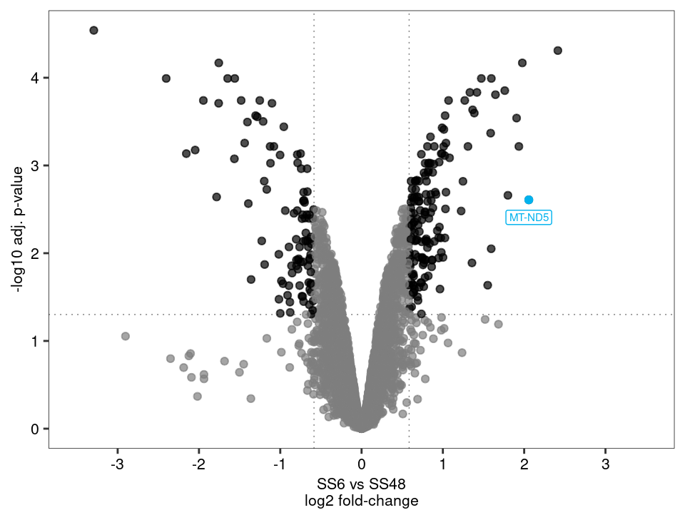
6 Volcano plotting
The most common way to visualise the results for a differential expression / abundance analysis is a volcano plot. We will use the fold-changes and adjusted p-values created by limma.
6.1 Static volcano plots
A static volcano plot is great for publications and presentations, ideally with some key target proteins highlighted and labelled. As an example, one upregulated protein is highlighted in the plot below.
Figure 5: A volcano plot highlights significantly changed proteins in an intuitive manner
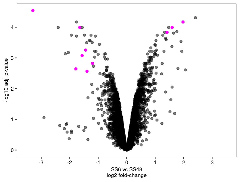
Let’s use this opportunity to visualise proteins that required imputation. If these proteins end up as extreme outliers, one could increase the stringency of the filtering or adjust the q and tune.sigma parameters of the imputation step.
Code
# Create a standard volcano plotpV2 <-ggplot(results, aes( x = log2_FC_SS6vsSS48, y =-log10(adj_p_value)))+geom_point(alpha =0.5)+geom_point(data = results[ !is.na(Imputed_samples) ], colour ="magenta")+scale_colour_manual(values =c("grey50", "black"))+scale_x_continuous(limits =c(-3.5, 3.5), breaks =seq(-4,4,1))+labs(x ="SS6 vs SS48\nlog2 fold-change", y ="-log10 adj. p-value")+theme(legend.position ="none")# Output plotpV2
Figure 6: Volcano plot highlighting proteins that required imputation (magenta). Extra care should be taken when interpreting these data points.
6.2 Interactive volcano plots
Volcano plots are often most useful for the initial data exploration. To be able to quickly check which proteins are up- and downregulated, we can create an interactive volcano plot. Clicking on a protein in this plot will automatically redirect users to its UniProt page, except for a handful of proteins that were not mapped to a single UniProt ID.
Code
# Prepare the data for highchartervolcano_data <- results[, .(Protein_group, gene_group, Genes, Protein_description, log2_FC_SS6vsSS48,pvalue_sci =formatC(adj_p_value, format ="e", digits =2), # Format p-values for tooltipneg_log10_pvalue =-log10(adj_p_value))] # Add a significant columnvolcano_data[, significance :=ifelse( abs(log2_FC_SS6vsSS48) >log2(FC_cutoff) & neg_log10_pvalue >-log10(pval_cutoff), "Significant", "Not Significant")]volcano_data[, significance :=factor(significance)]# Add a URL for UniProt, except for proteins were a group of genes was detectedvolcano_data[ !gene_group %like%";", url :=paste0("https://www.uniprot.org/uniprotkb/", gene_group)] # Generate the interactive volcano plotpHC <-hchart( volcano_data, "scatter", hcaes(x = log2_FC_SS6vsSS48, y = neg_log10_pvalue, group = significance)) %>%hc_chart( zoomType ="xy") %>%# Enables zooming on both x and y axeshc_xAxis( title =list(text ="SS6 vs SS48\nlog2 fold-change"), lineWidth =0.5, tickWidth =0.5, lineColor ="black", tickColor ="black", gridLineWidth =0 ) %>%hc_yAxis( title =list(text ="-log10 adj. p-value"), lineWidth =0.5, tickWidth =0.5, lineColor ="black", tickColor ="black", gridLineWidth =0 ) %>%hc_tooltip(headerFormat ="",pointFormat ="<b>{point.Genes}</b> | {point.Protein_group}<br>{point.Protein_description}<br>log2 FC: {point.log2_FC_SS6vsSS48:.2f}<br>p-value: {point.pvalue_sci}") %>%hc_plotOptions(scatter =list(marker =list(radius =3),states =list(hover =list(enabled =TRUE),inactive =list(enabled =FALSE)), # Don't dim inactive seriespoint =list(events =list( click =JS("function() { window.open(this.url, '_blank'); }"))))) %>%hc_colors(c("rgba(119,136,153, 0.7)", "rgba(33, 61, 90, 0.8)"))# Output plotpHC
Figure 7: Interactive volcano plot created using highcharter. Click on a point to be redirected to the protein’s UniProt page.
References
Lazar, Cosmin, Laurent Gatto, Myriam Ferro, Christophe Bruley, and Thomas Burger. 2016. “Accounting for the Multiple Natures of Missing Values in Label-Free Quantitative Proteomics Data Sets to Compare Imputation Strategies.”Journal of Proteome Research 15 (4): 1116–25. https://doi.org/10.1021/acs.jproteome.5b00981.
Peng, Hui, He Wang, Weijia Kong, Jinyan Li, and Wilson Wen Bin Goh. 2024. “Optimizing Differential Expression Analysis for Proteomics Data via High-Performing Rules and Ensemble Inference.”Nature Communications 15 (1). https://doi.org/10.1038/s41467-024-47899-w.
Ritchie, Matthew E, Belinda Phipson, Di Wu, Yifang Hu, Charity W Law, Wei Shi, and Gordon K Smyth. 2015. “Limma Powers Differential Expression Analyses for RNA-Sequencing and Microarray Studies” 43: e47. https://doi.org/10.1093/nar/gkv007.
---title: "Differential abundance analysis"subtitle: "Kustatscher lab tutorial"date: todayformat: htmllink-external-icon: truelink-external-newwindow: trueembed-resources: falsetoc: truenumber-sections: truetheme: light: cosmo dark: superherocode-tools: truecode-fold: truebibliography: references.bib---This is a reference workflow for differential abundance analysis, using a simple experiment comparing protein abundances across two cell lines (SS6 and SS48) with triplicate measurements. Workflow and code can be adapted to a wide range of proteomics experiments, such as time series or affinity purification experiments.::: {.callout-note appearance="minimal"}### How to follow this vignetteCopy the R code chunks and run them locally as you go through this document. You should already be familiar with R data.table and ggplot. The input file `protein_quant.csv.gz` is produced by the [DIA-NN data processing tutorial](https://diann-data-processing.netlify.app). The source code for this whole document is accessible through the Code button in the top right.:::## Preparing the data {#data_prep}We start with a data table of protein identifiers (e.g. `Protein_group`) and their quantities (e.g. `LFQ`) across samples. Initially, we prepare the data for downstream analysis (e.g. log2 transformation).```{r}#| message: false# Load required librarieslibrary(data.table); library(ggplot2); library(ggupset); library(patchwork); library(imputeLCMD); library(limma); library(highcharter)# Make script execution reproducibleset.seed(123)# Set a plotting theme for the whole documenttheme_set( theme( text =element_text(size =8), panel.border =element_rect(linewidth =0.25, colour ="black", fill =NA), panel.background =element_blank(), panel.grid =element_blank(), axis.text =element_text(colour ="black"), strip.background =element_blank(), strip.text =element_text(size =8, vjust =1)))# Load protein quantitationsDT <-fread("protein_quant.csv.gz")# Select a protein quantitation column (e.g. LFQ) and log2-transform itDT <- DT[, log2_quant :=log2(LFQ) ]# Print selected columnsDT[1:5, .(Sample, Protein_group, log2_quant)]```We also have a look at how many samples, conditions and replicates are available for this experiment:```{r}# Print sample, condition and replicate annotationDT[, .N, .(Sample, Condition, Replicate)]```## Filtering### SamplesOccasionally, an MS run may yield poor results, for example due to material loss during the sample prep. While we typically identify such outliers earlier in the data processing pipeline, it is good practice to perform a PCA analysis to identify any samples that deviate unexpectedly. Another flag for problematic runs is a severe drop in the number of quantified proteins. As shown by @fig-PCA_and_bar, there are no obvious outliers in this dataset and no samples need to be excluded.```{r}#| label: fig-PCA_and_bar#| fig-cap: "Inspecting dataset for outlier samples. (A) PCA shows that replicates group together as expected. (B) Bar chart shows consistent number of proteins identified across replicates."#| fig-height: 3# Run a PCA to check for major trendsPCA_input <-dcast(DT, Protein_group ~ Sample, value.var ="log2_quant") # Cast into a wide data format for PCA analysisPCA_input <- PCA_input[ complete.cases(PCA_input) ] # Can't do PCA with missing valuesPCA_input <-t( data.frame( PCA_input, row.names ="Protein_group" )) # Convert to dataframe and transpose to compare samplesDT_PCA <-prcomp( PCA_input , scale. =TRUE ) # Run PCAvar_explained <-summary(DT_PCA)$importance # Extract variance explainedDT_PCA <-data.table(DT_PCA$x, keep.rownames ="Sample") # Prepare for plottingDT_PCA <-merge(DT_PCA, unique(DT[, .(Sample, Condition, Replicate)])) # Add annotation of conditions and replicates# Create PCA plotpPCA <-ggplot(DT_PCA, aes(x = PC1, y = PC2, colour = Condition, shape = Replicate))+geom_point( size =2 )+scale_colour_brewer(palette ="Set1")+xlab(paste("PC1 [", round( var_explained[ rownames(var_explained) =="Proportion of Variance" , "PC1"] *100, 0), "%]", sep =""))+ylab(paste("PC2 [", round( var_explained[ rownames(var_explained) =="Proportion of Variance" , "PC2"] *100, 0), "%]", sep =""))+theme(axis.text =element_blank(), axis.ticks =element_blank(), legend.title =element_blank())# Create barplot with number of remaining proteins per samplepBar <-ggplot( DT[, .N, .(Condition, Replicate)], aes( x = Condition, y = N, fill = Replicate, label = N))+geom_bar(stat ="identity", position ="dodge2")+geom_text(position =position_dodge2(width =0.9), vjust =0.5, hjust =1.2, size =3, angle =90)+scale_fill_brewer()+labs(x =NULL, y ="Protein count", fill =NULL)# Arrange the two plots into a single figure using the Patchwork packagefree(pPCA, type ="label") + pBar +plot_annotation(tag_levels ="A")```### Proteins {#prot_filter}We filter out proteins with insufficient or unreliable quantitation, aiming to retain as many as possible for downstream analysis while minimising noise from inconsistently measured proteins. There is no single filtering strategy that will work for all datasets. The filtering strategy needs to be tailored to the data and the downstream analysis. Generally, it helps to consider both quality (e.g. number of precursors) and frequency (e.g. number of replicates) of protein quantitations.This particular dataset has six samples. We filter it as follows:- Keep proteins detected in all 6 samples with at least 2 precursors (n = 6,310).- Keep proteins detected in 5 samples with at least 3 precursors. We can still calculate fold-changes and p-values for these proteins, but significance will be reduced due to the missing replicate in one condition. The stricter precursor threshold reduces the risk of retaining spurious hits (n = 13).- We *cannot* keep proteins detected in ≤4 samples, because the resulting statistical analysis would be unreliable. An important exception is when a protein is consistently quantified in all replicates of one condition but entirely absent in the other. This could be a truly condition-specific expression profile, or a highly specific interaction in an IP compared to an IgG control. In such cases, we can impute a baseline value for the missing condition, allowing us to calculate a fold-change for statistical analysis (see [imputation](#NA_imp) section). Any such fold-change will be a conservative estimate compared to the "infinite" fold-change implied by a complete absence in one condition. To capture this third group, we keep proteins detected in 3 samples with at least 5 precursors, but only if the three samples belong to the same condition, and only if they were not detected at all in the other condition (n = 9).After filtering, let's see how many proteins we have left to work with:```{r}#| label: fig-upset#| fig-cap: "Protein numbers after filtering, and their overlap across samples."#| warning: false#| fig-height: 3# Calculate protein stats before filteringprotein_stats <- DT[, .(n_samples = .N, # Number of samplesmin_precursors =min(N_precursors), # Mininum number of precursors across samplesn_conditions =uniqueN(Condition) # Number of different conditions ), Protein_group ] # Calculate for each protein# Proteins detected in 6 samples with at least 2 precursorskeepers_1 <- protein_stats[ n_samples ==6& min_precursors >=2, Protein_group ]# Proteins detected in 5 samples with at least 3 precursorskeepers_2 <- protein_stats[ n_samples ==5& min_precursors >=3, Protein_group ]# Proteins detected in 3 samples with at least 4 precursors, but these samples are from a single condition, and the protein has not been detected at all in the other conditionkeepers_3 <- protein_stats[ n_samples ==3& min_precursors >=5& n_conditions ==1, Protein_group]# Filter table to keep only these three sets of proteinsDT <- DT[ Protein_group %in%c(keepers_1, keepers_2, keepers_3) ]# Create UpSet plot to show protein overlap between sample pairspUpSet <-ggplot( DT[, .(Sample =list(Sample)), by = Protein_group], # Prep data for ggupset's scale_x_upset functionaes(x = Sample))+geom_bar()+geom_text(stat='count', aes(label =after_stat(count)), vjust =-0.5, size =3) +# This adds protein numbers on top of the barsscale_x_upset(order_by ="degree", reverse =TRUE, sets = DT[ order(Condition), unique(Sample)] )+# Explicitly providing the set names allows us to order them by conditionlabs(x =NULL, y ="Protein count")+scale_y_continuous(expand =expansion(mult =c(0,0.15))) # This expansion is necessary to accomodate numbers on top of bars# Output plotpUpSet```## NormalisationThese data have already been normalised at the precursor level to adjust for unequal sample loading. Additional normalisation steps are often not required. In fact, some sophisticated normalisation procedures used in the field are actually reducing workflow performance [@Peng2024]. Nevertheless, for many experiments we can assume that most protein abundances do not change between conditions, so we set the median protein abundance to the same value across all samples.```{r}#| label: fig-normalisation#| fig-cap: "Boxplot showing protein quantities before and after median-normalisation. Median normalisation helps to make sure that the median fold-change between conditions is zero."#| fig-height: 3# Identify the "median of the medians". This will become the new median for all samples.target_median <- DT[, median(log2_quant), Sample][, median(V1)]# Scale protein quantities to obtain this target_median for all samplesDT[, log2_quant_norm := log2_quant -median(log2_quant) + target_median, by = Sample] # Plot the values before and after the median normalisationpBar <-ggplot( data =melt(DT, measure.vars =c("log2_quant", "log2_quant_norm")),aes(x = Condition, fill = Replicate, y = value))+facet_wrap("variable", labeller =labeller(variable =c("log2_quant"="before", "log2_quant_norm"="after")))+geom_boxplot(outliers =FALSE)+scale_fill_brewer()+labs(x =NULL, y ="log2 protein quantities")# Output plotpBar```## Missing value imputation {#NA_imp}Missing values are common in proteomics and many algorithms exist to impute them. However, imputation should be used very cautiously. Most missing values in proteomics are missing for a reason, typically because low-abundance proteins are inconsistently quantified across samples. In many cases, imputation is not necessary. For example, proteins quantified in 5 samples in this dataset (`keepers_2`) are missing from one replicate in one condition. We can calculate differential expression p-values for such proteins (see [below](#daa)), which will be less significant than for comparable proteins with a full set of replicates. Nevertheless, this is a more robust approach than imputing a value for the missing replicate and feeding it as "real" observation into the differential expression analysis.However, there is one scenario where imputation is necessary: when a protein is consistently and robustly detected in one condition but entirely absent in another (see [protein filtering](#prot_filter) section). In our dataset we have identified 9 proteins that may considered truly condition-specific (`keepers_3`). For these proteins, we can impute "baseline" values for the condition in which they are absent, so that we can estimate fold-changes and include them in our downstream analysis.We use the [minProb](https://www.rdocumentation.org/packages/imputeLCMD/versions/2.0/topics/impute.MinProb) approach, which simulates low-abundance values in a sample- and protein-specific manner [@Lazar2016]. Specifically, minProb draws a random value from a normal distribution, where the mean corresponds to the bottom 1% of intensities in the sample. The distribution's variance is determined by the variability of the protein's abundances in the samples where it was detected.```{r}#| label: fig-imputation-1#| results: hide#| fig-cap: The values imputed by MinProb fall towards the bottom end of the distribution of the measured values. To change the position or width of the imputed data distribution, adjust q and tune.sigma, respectively. Note we only actually impute values for 9 proteins.#| fig-width: 4#| fig-height: 2.5# We first need to cast the data into a wide formatwDT <-dcast(DT, Protein_group ~ Sample, value.var ="log2_quant_norm", fill =NA)# Impute missing values wDT_imp <-impute.MinProb( as.matrix(wDT, rownames ="Protein_group"), q =0.01, tune.sigma =1) # Turn imputed data back into a data.tablewDT_imp <-as.data.table(wDT_imp, keep.rownames ="Protein_group")# Create a table that allows the identification of the original and imputed valuesplot_imp_dt <-merge(melt(wDT, id.vars ="Protein_group", value.name ="measured_val" ),melt(wDT_imp, id.vars ="Protein_group", value.name ="imputed_val" ))plot_imp_dt[ is.na(measured_val), data :="imputed" ]plot_imp_dt[ !is.na(measured_val), data :="measured" ]# Visualise the distribution of the imputed data using this tableggplot( plot_imp_dt, aes(imputed_val, fill = data))+geom_density(adjust =2, alpha =0.5)+labs(x ="Normalised LFQ intensity", y ="Density", fill =NULL)```Note that `wDT_imp` contains imputed data for *all* missing values (we had to supply the whole data set for imputation, because MinProb needs to know the overall distribution of the data). However, we only want to impute the values for proteins that were exclusively detected in one condition, which we had previously defined as `keepers_3`. We therefore need to swap out that subsection of our data matrix with the corresponding imputed section.```{r}#| label: fig-imputation-2# Make a record of which values exactly were imputedimpNAs <-melt( wDT[ Protein_group %in% keepers_3 ], id.vars ="Protein_group" )impNAs <- impNAs[ is.na(value), .(Imputed_samples =paste(variable, collapse =",")), Protein_group ]# Replace the original values for these proteins with the imputed oneswDT <-rbindlist( list( wDT[ !Protein_group %in% keepers_3 ], wDT_imp[ Protein_group %in% keepers_3 ]), use.names =TRUE )```## Differential abundance analysis {#daa}### Using a t-testWe first calculate log2 fold-changes manually and use a simple t-test to assess if there is a significant difference between the two conditions. This is a straightforward approach, and in many cases it is sufficient.```{r}#| label: DAA_by_t_test# Melt the partially imputed data matrix into long-formatmDT <-melt( wDT, id.vars ="Protein_group", value.name ="log2_quant_norm", variable.factor =FALSE, variable.name ="Sample", na.rm =TRUE)# Re-annotate conditionsmDT[, Condition :=gsub("R\\d_", "", Sample)] # Un-log the LFQ intensities to calculate mean and CVsmDT[, quant_norm :=2^log2_quant_norm ]# For each protein and condition, calculate mean, CV and number of replicates per conditionFC <- mDT[, .(log2_mean_LFQ =log2( mean( quant_norm )), # Log2 of arithmetic mean of LFQsCV =sd(quant_norm) /mean(quant_norm) *100, # CV values across replicatesN_replicates = .N # Number of replicates ), .(Protein_group, Condition) ]# Cast back into a wide tableFC <-dcast(FC, Protein_group ~ Condition, value.var =c("log2_mean_LFQ", "CV", "N_replicates"))# Calculate log2 fold-changeFC[, manual_log2_FC_SS6_SS48 := log2_mean_LFQ_SS6 - log2_mean_LFQ_SS48 ]# Calculate p-values for differential abundance using a t.test (it is generally recommended to do this in log-space)pvalues <- mDT[, .(pval_t_test =t.test(log2_quant_norm ~ Condition)$p.value), Protein_group]# Combine fold-changes and p-valuesFC <-merge(FC, pvalues, by ="Protein_group")# Print resulting data frameFC[ 1:5, .(Protein_group, manual_log2_FC_SS6_SS48, pval_t_test, CV_SS6, CV_SS48)]```### Using LimmaLimma is a more sophisticated approach for differential expression analysis [@limma-2]. Originally developed for microarrays, it offers two key advantages over a t-test. Limma can handle complex experimental setups, such as comparing multiple conditions and time points, and it can even model and adjust for batch effects. In addition, limma performs particularly well in studies with small sample sizes. With only 3-4 replicates, the true expression variation of a gene is difficult to estimate, which can lead to unreliable p-values. Limma addresses this using an empirical Bayes approach to "borrow information" across all genes. This leads to more stable estimates of expression variability, and therefore more reliable identification of differentially expressed genes. Here we outline a basic limma experiment. For more information, see limma vignettes[^1].[^1]: Useful resources on limma: - [User guide](https://bioconductor.org/packages/release/bioc/html/limma.html) - [Vignette on design and contrast matrices](https://bioconductor.org/packages/release/workflows/vignettes/RNAseq123/inst/doc/designmatrices.html)First, we need to create a design matrix. It tells limma which MS runs / samples (rows) belong to which experimental condition (columns). It is a standard numeric matrix in R, with 1 indicating a match, and zero indicating no match. Design matrices can become quite complex for advanced experimental designs.```{r}#| label: limma-design# Extract a table that maps samples to conditions sample_map <-unique( DT[, .(Sample, Condition)] )# Turn into design matrix of 1s (match) and 0s (no match). The model.matrix function is made for this, but not very intuitive.design <-model.matrix( ~0+ Condition, data = sample_map)# Adjust the column and row namescolnames(design) <-gsub("Condition", "", colnames(design))rownames(design) <- sample_map$Sample# Set the order of the columns in wDT to match the design matrix. This is critical because limma matches them by position, not by namesetcolorder(wDT, neworder =c("Protein_group", sample_map$Sample))# Print design matrixdesign ```Next, we fit the linear model. The present data set is very simple, so only one comparison (SS6 vs SS48) is relevant, but for experiments with multiple conditions (e.g. WT, mutant1, mutant2, mutant3), we could extract multiple pairwise comparisons. These comparisons are called contrasts. We can define a set of contrasts of interest using a contrast matrix. For example, the contrast `SS6-SS48` will calculate the log2 fold-change and p-values for SS6 / SS48. We then apply the empirical Bayes method to adjust the protein variances (`eBayes`). Finally, we extract the relevant information from the linear model fit using `topTable`.```{r}#| label: limma-calc#| message: false# Fit the linear modelfit <-lmFit(wDT, design)# Define a contrast matrix and extract contrastscont.matrix <-makeContrasts( SS6vsSS48 = SS6-SS48, levels = design)fit2 <-contrasts.fit(fit, cont.matrix)# Borrow information across all proteins to adjust variance estimatesfit2 <-eBayes(fit2)# Extract the limma results, including p-value adjustmentFC_limma <-topTable(fit2, adjust="BH", number =Inf)# Convert the output to data.table, keep and re-name relevant columns and print on screenFC_limma <-as.data.table(FC_limma)FC_limma <- FC_limma[, .(Protein_group, log2_FC_SS6vsSS48 = logFC, p_value = P.Value, adj_p_value = adj.P.Val)]FC_limma[ 1:5 , .(Protein_group, log2_FC_SS6vsSS48, p_value, adj_p_value) ]```We can now combine all results and annotation data to create an overall output file for our differential abundance analysis.```{r}# Merge manual and limma-based differential abundance dataresults <-merge(FC, FC_limma, by ="Protein_group")# Add the annotation about which values were imputedresults <-merge(results, impNAs, by ="Protein_group", all.x =TRUE)# Add gene and protein namesresults <-merge(results, unique( DT[, .(Protein_group, Genes, Protein_description)] ), by ="Protein_group")# Add additional summary statisticssum_stat <- DT[, .( min_N_precursors =min(N_precursors),min_N_precursors_proteotypic =min(N_precursors_proteotypic) ), .(Protein_group, Condition)]sum_stat <-dcast(sum_stat, Protein_group ~ Condition, value.var =c("min_N_precursors", "min_N_precursors_proteotypic"))results <-merge(results, sum_stat, by ="Protein_group", all.x =TRUE)# Extract gene-level UniProt IDs to merge the data with gene-level annotation later on.# This means removing protein isoform information. Gene-level IDs are not unique.results[, gene_group :=sapply(strsplit(Protein_group, ";"), # (1) Split each Protein_group into individual UniProt IDsfunction(x){paste( # (4) If there are multiple genes, combine them back into a group, separated by ;unique( # (3) If there were multiple isoforms, keep only the unique gene-level IDgsub("-.+", "", x) # (2) Remove isoform information (e.g., "-2") from each UniProt ID ), collapse =";") } )]# Set the order of columns in the final outputsetcolorder(results, neworder =c(1, 20, 14, 15, 13, 2:7, 16:19))# Write out the result filefwrite(results, "DAA_results.csv.gz")```::: {.callout-note collapse="true"}## Brief explanation of output columns- Protein_group: Uniprot IDs, the main identifier column- gene_group: Same as Protein_group, but isoform-annotation removed. Use this for gene-level annotation.- Genes: Gene names. Not unique, use only for labelling plots.- Protein_description: Short description of protein.- Imputed_samples: Lists the imputed samples (for proteins with imputation only)- log2_mean_LFQ_SS48 / \_SS6: Log2 of average LFQ per condition- CV_SS48 / \_SS6: Coefficient of variation per condition- N_replicates_SS48 / \_SS6: Number of replicates per condition- min_N_precursors_SS48 / \_SS6: Minimum number of precursors across all replicates- min_N_precursors_proteotypic_SS48 / \_SS6: Same for proteotypic precursors- manual_log2_FC_SS6_SS48: Arithmetic log2 fold-change between conditions (manual)- pval_t_test: P-value from t-test between conditions (manual)- log2_FC_SS6vsSS48: Limma estimate of log2 fold-change between conditions- p_value: P-value from limma- adj_p_value: BH-adjusted P-value from limma:::Fold-changes calculated by limma differ slightly from the manually calculates ones, especially for proteins with high CV values. This is because limma uses a model to estimate fold-changes, which takes data variability into account. Limma p-values are generally more significant than those from t-tests, so that it is possible to adjust them for multiple comparisons and still detect many significant abundance changes. Limma p-values also reflect the protein fold-change more accurately, with smaller fold-changes producing less significant p-values, especially for proteins with fewer replicate measurements. In short, the limma-derived metrics outperform the "manual" versions.## Volcano plottingThe most common way to visualise the results for a differential expression / abundance analysis is a volcano plot. We will use the fold-changes and adjusted p-values created by limma.### Static volcano plotsA static volcano plot is great for publications and presentations, ideally with some key target proteins highlighted and labelled. As an example, one upregulated protein is highlighted in the plot below.```{r}#| label: fig-volcano-static#| fig-align: center#| fig-width: 5#| fig-height: 3.8#| fig-cap: "A volcano plot highlights significantly changed proteins in an intuitive manner"# Define cut-offs for plottingFC_cutoff <-1.5pval_cutoff <-0.05# Create a standard volcano plotpV1 <-ggplot( results,aes( x = log2_FC_SS6vsSS48, y =-log10(adj_p_value), colour =abs(log2_FC_SS6vsSS48) >log2(FC_cutoff) & adj_p_value < pval_cutoff,label = Genes))+geom_hline( yintercept =-log10(pval_cutoff), linetype ="dotted", colour ="grey50", linewidth =0.25)+geom_vline( xintercept =c(-log2(FC_cutoff), log2(FC_cutoff)), linetype ="dotted", colour ="grey50", linewidth =0.25)+geom_point(alpha =0.7)+geom_point(data = results[ Protein_group =="P03915"], colour ="deepskyblue2")+geom_label(data = results[ Protein_group =="P03915"], colour ="deepskyblue2", size =2, nudge_y =-0.2 )+scale_colour_manual(values =c("grey50", "black"))+scale_x_continuous(limits =c(-3.5, 3.5), breaks =seq(-4,4,1))+labs(x ="SS6 vs SS48\nlog2 fold-change", y ="-log10 adj. p-value")+theme(legend.position ="none")# Output plotpV1 ```Let's use this opportunity to visualise proteins that required imputation. If these proteins end up as extreme outliers, one could increase the stringency of the filtering or adjust the `q` and `tune.sigma` parameters of the imputation step.```{r}#| label: fig-volcano-static-imputed#| fig-align: center#| fig-width: 5#| fig-height: 3.8#| fig-cap: "Volcano plot highlighting proteins that required imputation (magenta). Extra care should be taken when interpreting these data points."# Create a standard volcano plotpV2 <-ggplot(results, aes( x = log2_FC_SS6vsSS48, y =-log10(adj_p_value)))+geom_point(alpha =0.5)+geom_point(data = results[ !is.na(Imputed_samples) ], colour ="magenta")+scale_colour_manual(values =c("grey50", "black"))+scale_x_continuous(limits =c(-3.5, 3.5), breaks =seq(-4,4,1))+labs(x ="SS6 vs SS48\nlog2 fold-change", y ="-log10 adj. p-value")+theme(legend.position ="none")# Output plotpV2```### Interactive volcano plotsVolcano plots are often most useful for the initial data exploration. To be able to quickly check which proteins are up- and downregulated, we can create an interactive volcano plot. Clicking on a protein in this plot will automatically redirect users to its UniProt page, except for a handful of proteins that were not mapped to a single UniProt ID.```{r}#| label: fig-volcano-interactive#| layout: [[-10,75,-15]]#| fig-cap: "Interactive volcano plot created using highcharter. Click on a point to be redirected to the protein's UniProt page."# Prepare the data for highchartervolcano_data <- results[, .(Protein_group, gene_group, Genes, Protein_description, log2_FC_SS6vsSS48,pvalue_sci =formatC(adj_p_value, format ="e", digits =2), # Format p-values for tooltipneg_log10_pvalue =-log10(adj_p_value))] # Add a significant columnvolcano_data[, significance :=ifelse( abs(log2_FC_SS6vsSS48) >log2(FC_cutoff) & neg_log10_pvalue >-log10(pval_cutoff), "Significant", "Not Significant")]volcano_data[, significance :=factor(significance)]# Add a URL for UniProt, except for proteins were a group of genes was detectedvolcano_data[ !gene_group %like%";", url :=paste0("https://www.uniprot.org/uniprotkb/", gene_group)] # Generate the interactive volcano plotpHC <-hchart( volcano_data, "scatter", hcaes(x = log2_FC_SS6vsSS48, y = neg_log10_pvalue, group = significance)) %>%hc_chart( zoomType ="xy") %>%# Enables zooming on both x and y axeshc_xAxis( title =list(text ="SS6 vs SS48\nlog2 fold-change"), lineWidth =0.5, tickWidth =0.5, lineColor ="black", tickColor ="black", gridLineWidth =0 ) %>%hc_yAxis( title =list(text ="-log10 adj. p-value"), lineWidth =0.5, tickWidth =0.5, lineColor ="black", tickColor ="black", gridLineWidth =0 ) %>%hc_tooltip(headerFormat ="",pointFormat ="<b>{point.Genes}</b> | {point.Protein_group}<br>{point.Protein_description}<br>log2 FC: {point.log2_FC_SS6vsSS48:.2f}<br>p-value: {point.pvalue_sci}") %>%hc_plotOptions(scatter =list(marker =list(radius =3),states =list(hover =list(enabled =TRUE),inactive =list(enabled =FALSE)), # Don't dim inactive seriespoint =list(events =list( click =JS("function() { window.open(this.url, '_blank'); }"))))) %>%hc_colors(c("rgba(119,136,153, 0.7)", "rgba(33, 61, 90, 0.8)"))# Output plotpHC```